EDGE DETECTION – FUNDAMENTALS

The derivatives of a digital function are defined in terms of differences.

The above statement made me to analyze about derivatives and how it is used for edge detection.  The first time when I came across the edge detection operation [Example: edge(Image,’sobel’)], I wondered how it worked. 

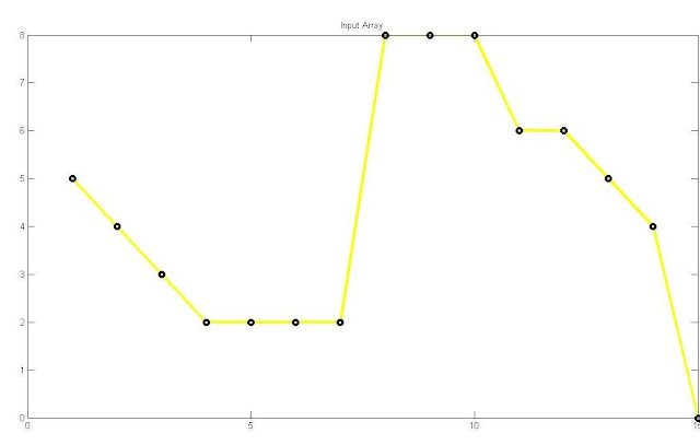
Consider a single dimensional array,

A =

5

4

3

2

2

2

2

8

8

8

6

6

5

4

0

MATLAB CODE:

x=1:15;

y=[5 4 3 2 2 2 2 8 8 8 6 6 5 4 0];

figure,

plot(x,y,'-o','LineWidth',3,'MarkerEdgeColor','k','Color','y');

title('Input Array');

First-order Derivative for one dimensional function f(x):

MATLAB  CODE:

x1=1:14;

y1=diff(y,1);

figure,

plot(x1,y1,'-o','LineWidth',3,'MarkerEdgeColor','k','Color','r');

-1

-1

-1

0

0

0

6

0

0

-2

0

-1

-1

-4

NOTE: The contiguous values are zero. Since the values are nonzero for non-contiguous values, the result will be thick edges.

The first-order derivative produces thicker edges.

Second-order Derivative for one dimensional function f(x):

MATLAB CODE:

x2=1:13;

y2=diff(y,2);

figure,

plot(x2,y2,'-o','LineWidth',3,'MarkerEdgeColor','k','Color','g');

0

0

1

0

0

6

-6

0

-2

2

-1

0

-3

The Second-order derivative gives finer result compared to first-order derivative. It gives fine detailed thin lines and isolated points.  Let’s see how the second-order derivative used for Image sharpening (Laplacian) in my upcoming post.