Digital Image Water Marking – Part 1

Digital image watermarking is the method in which data is embedded in a multimedia file such as an image or a video, so as to verify the credibility of the content or the identity of the owner.

MATLAB CODE:

%Digital Image Watermarking

%Unmasked Image f

f = imread('angel.jpg');

figure,imshow(f);title('Unmasked Image');

 

Unmasked Image

%Watermark

w = imread('watermark_sym.jpg');

figure,imshow(w);title('Watermark');

%Visibility of the watermark

alpha=0.5;

Fw = (1-alpha)*f + alpha.*w;

figure,imshow(Fw);title('Watermarked Image-Visibilty:0.5');

Explanation:

1.      Read the image to be watermarked. In my case it ‘s ‘angel.jpg’

2.      Read the watermark. Make sure the image size and the watermark size are same.

3.      Adjust the alpha value based on your requirement. Alpha can be between 0 and 1. If alpha is less than 0.5 the watermark will be less visible and if the alpha is more than 0.5, the watermark will be clearly visible.

MATLAB CODE:

%Read the Blog logo

Logo = imread('Dwatermark2.jpg');

figure,imshow(Logo);title('Blog Logo');

OIm = f;

%Visibility control

alpha = 0.5;

[m, n,~]=size(Logo);

%choose a portion of the Image

Sz = [495 927];

%Apply watermark

OIm(Sz(1):Sz(1)+m-1,Sz(2):Sz(2)+n-1,:)=(1-alpha)*OIm(Sz(1):Sz(1)+m-1,Sz(2):Sz(2)+n-1,:) + alpha.*Logo;

figure,imshow(OIm);title('Watermark in the centre');

EXPLANATION:

1.      Read the blog logo.

2.      Note: The size of the input image and the logo are not same.

3.      Choose a portion in the input image and apply watermark.

LSB Digital Watermarking

In this method, the watermark is hidden in the input image.

Consider a pixel from the input image; say 249 and a pixel from the watermark say, 155.

Now hide the pixel value of the watermark in the two least significant bits of the input image.

1.      The binary representation of 249 is 11111001

2.      The binary representation of 155 is 10011011

3.      Make the two least significant bits of input image value 249 to zeros i.e. 11111000

4.      Find the two Most significant bits of the watermark value 155 i.e. 10

5.      Now place the two most significant bits of the watermark at the two least significant bits of the input image.

6.      11111000 + 00000010= 11111010 i.e.  250

MATLAB CODE:

%LSB watermarked Image

Fw1 = 4*(f/4) + w/64;

figure,imshow(Fw1);title('LSB watermarked Image');

How to retrieve the watermark:

Method 1:

Subtract the input image (without watermark) from the watermarked Image.

%Retrieve the Watermark

DMark = (Fw1-f)*64;

figure,imshow(DMark);title('Watermark extracted from the image');

Method 2:

Retrieve the two least significant bits of the image

%Retrieve the Watermark

DMark2 = rem(Fw1,4)*64;

figure,imshow(DMark2);title('Watermark extracted from the image');

We can extend the above techniques for steganography or image coding. In the next upcoming post I will share about how to validate the digital watermark.

Image Zooming – Part 1

Let’s try to view an Image of size 1366 x 768.

To view the image:

I = imread('Vatican-City-Wallpaper_.jpg');

figure,imshow(I);

Reference:

Vatican City Wallpaper - HD Wallpapers

The image is too big. I want to view the image part by part, so that I can view the details in the image more clearly.

Method one:

I use MATLAB function ‘imshow’ and the ‘figure’ command.

To view the image:

I = imread('Vatican-City-Wallpaper_jpg');

figure,imshow(I);

Now click the ‘zoom in’ option to enlarge the image.

ZOOM IN

Click the ‘pan’ option and drag the cursor to view the image part by part.

 

PAN OPTION

Method two:

We can do the image viewing using our own code instead of using ‘zoom in’ and ‘pan’ options.

We will define our own window and display the image alone.

%Read the Image

I=imread('Vatican-City-Wallpaper_.jpg');

Im=I;

%Get the Screen size and define the window

scrsz = get(0,'ScreenSize');

figure('Position',[300 50 scrsz(3)-600 scrsz(4)-200],'Menu','none','NumberTitle','off','Name','VIEW PHOTO','Resize','off');

%Size of the Image Portion

Len=round(size(I,1)/4);

Flag=1;

x=1;

wid=Len;

y=1;

ht=Len;

%Display the image

ax=axes('Position',[0 .1 1 .8],'xtick',[],'ytick',[]);

imshow(Im(x:wid,y:ht,:));

Num=50;

while(Flag==1)

try

    %User button click

    waitforbuttonpress;

    pt=get(ax,'CurrentPoint');

    y1=round(pt(1,1));

    x1=round(pt(1,2));

   

    %Calculate the Next part of the image based on the button press

    if( x1 < Len && x1 > 0 && y1 < Len && y1 > 0)

   

    x=x+x1;

    y=y+y1;

    if(x-Num>1)

      

        x=x-Num;

    end

   

    if(y-Num>1)

      

        y=y-Num;

    end

   

    if(x+wid>size(I,1))

      

        x=size(I,1)-wid;

    end

   

    if(y+ht>size(I,2))

      

        y=size(I,2)-ht;

    end

   %New Image Part

   imshow(Im(x:x+wid,y:y+ht,:));

  

   wid=Len;

   ht=Len;

  

    end

catch

    Flag=0;

end

end

 

Click on the bottom right part of the image to view the center part

Click to the right from the above mentioned part 

Gaussian Filter without using the MATLAB built_in function

Gaussian Filter

Gaussian Filter is used to blur the image. It is used to reduce the noise and the image details.

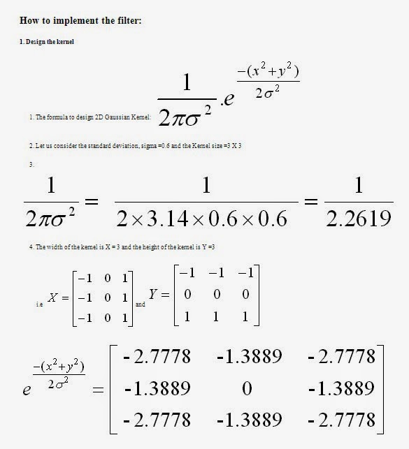
          The Gaussian kernel's center part  ( Here 0.4421 )  has the highest value and  intensity of other pixels                 decrease as the distance from the center part increases.

               On convolution of the local region and the Gaussian kernel gives the highest intensity value to the center part of the local region(38.4624) and the remaining pixels have less intensity as the distance from the center increases.
               Sum up the result and store it in the current pixel location(Intensity = 94.9269) of the image.

MATLAB CODE:

%Gaussian filter using MATLAB built_in function

%Read an Image

Img = imread('coins.png');

A = imnoise(Img,'Gaussian',0.04,0.003);

%Image with noise

figure,imshow(A);

H = fspecial('Gaussian',[9 9],1.76);

GaussF = imfilter(A,H);

figure,imshow(GaussF);

MATLAB CODE for Gaussian blur WITHOUT built_in function:

%Read an Image

Img = imread('coins.png');

A = imnoise(Img,'Gaussian',0.04,0.003);

%Image with noise

figure,imshow(A);

 

Image with Noise

I = double(A);

%Design the Gaussian Kernel

%Standard Deviation

sigma = 1.76;

%Window size

sz = 4;

[x,y]=meshgrid(-sz:sz,-sz:sz);

M = size(x,1)-1;

N = size(y,1)-1;

Exp_comp = -(x.^2+y.^2)/(2*sigma*sigma);

Kernel= exp(Exp_comp)/(2*pi*sigma*sigma);

 

Gaussian Kernel 9x9 size with Standard Deviation =1.76

%Initialize

Output=zeros(size(I));

%Pad the vector with zeros

I = padarray(I,[sz sz]);

%Convolution

for i = 1:size(I,1)-M

    for j =1:size(I,2)-N

        Temp = I(i:i+M,j:j+M).*Kernel;

        Output(i,j)=sum(Temp(:));

    end

end

%Image without Noise after Gaussian blur

Output = uint8(Output);

figure,imshow(Output);

After Filtering

Lossless Predictive coding - MATLAB CODE

A new pixel value is obtained by finding the difference between the current pixel and the predicted pixel value.

Encoding:

STEPS TO BE PERFORMED:

MATLAB CODE:

clear all

clc

%Read the input image

% A=imread('rice.png');

% figure,imshow(A);

% A=double(A);

A=[10 2 3 4;5 6 7 8];

display(A);

e=A;

%Perform prediction error

for i = 1:size(A,1)

    for j = 2:size(A,2)

        e(i,j)=e(i,j)-A(i,j-1);

    end

end

display(e);

%Huffman coding

C=reshape(e,[],1);

[D1,x]=hist(C,min(min(e)):max(max(e)));

sym=x(D1>0);

prob=D1(D1>0)/numel(e);

[dict,avglen] = huffmandict(sym,prob);

comp = huffmanenco(C,dict);

%Huffman Decoding

dsig = huffmandeco(comp,dict);

e=reshape(dsig,size(A,1),size(A,2));

d=e;

for i = 1:size(A,1)

    for j = 2:size(A,2)

        d(i,j)=d(i,j-1)+e(i,j);

    end

end

display(d);

%Decompressed Image

%figure,imshow(uint8(d));

2-D Prediction:

Consider an array [ a  b

                    c  d]

To perform prediction error using 2-D linear operator, e(2,2)=d-(c+b) i.e subtract the pixels left and top to the current pixel

To decompress, perform inverse operation f(2,2)=d+(c+b)

MATLAB CODE:

clear all

clc

%Input sequence

A=[10 11 12 13; 2 14 26 39];

display(A);

e=A;

A1=padarray(A,[1,0],0);

%Prediction error

for i = 2:size(A1,1)-1

    for j = 2:size(A1,2)

        fx=round(A1(i,j-1)+A1(i-1,j));

         e(i-1,j)=e(i-1,j)-fx;

    end

end

display(e);

%Huffman encoding

C=reshape(e,[],1);

[D1,x]=hist(C,min(min(e)):max(max(e)));

sym=x(D1>0);

prob=D1(D1>0)/numel(e);

[dict,avglen] = huffmandict(sym,prob);

comp = huffmanenco(C,dict);

%Huffman decoding

dsig = huffmandeco(comp,dict);

e=reshape(dsig,size(A,1),size(A,2));

%Inverse operation

d=e;

e1=padarray(e,[1,0],0);

for i = 2:size(e1,1)-1

    for j = 2:size(e1,2)

        fx=round(e1(i,j-1)+e1(i-1,j));

        d(i-1,j)=d(i-1,j)+fx;

        e1=padarray(d,[1,0],0);

    end

end

display(d);

  

A is the input value, e is the encoded value, d is the decoded value

Basic Intensity Transformation Functions – Part 1

Basic Intensity Transformation Functions – Part 1

Three basic types of functions used for image Enhancement are:

1.       Linear transformation

2.       Logarithmic transformation

3.       Power Law transformation

Consider an Image r with intensity levels in the range [0 L-1]

1.       Image Negatives

Equation : s = L – 1 – r

Consider  L  = 256 and r be the intensity of the image(Range 0 to 255)

MATLAB CODE:

A=imread('rice.png');

figure,imshow(A);title('Original Image');

%Image Negative

L=256;

s= (L-1)-A;

figure,imshow(s);title('Image negative -> S = L - 1 - r')

EXPLANATION:

Consider array r = [ 1 10 255 100]

  S = 256 – 1 – r gives [ 254 245 0 155]

2.       Log Transformation

Equation: s = c log(1 + r) where c is a constant

Consider  c = 1 and r be the intensity of the image(Range 0 to 255)

MATLABCODE:

%Log Transformation

%Input Image in type double

r=double(A);

C=1;

S=C*log(1+r);

Temp=255/(C*log(256));

%Display image range [0 255]

B=uint8(Temp*S);

figure,imshow(B);title('Log Transformation -> S = clog(1+r)');

EXPLANATION:

a.       Convert the image to type double

b.      Apply the log transformation

c.       Map the obtained values to the range [0 255]

3.       Power –Law (Gamma) corrections

Equation :

Where c and gamma are positive constants

Consider c = 1, gamma =0.04 and r be the intensity of the image (Range 0 to 255)

MATLAB CODE:

G=0.40;%Gamma =0.40

S=C*(r.^G);

Temp=255/(C*(255.^G));

%display image range [0 255]

S1=uint8(Temp*S);

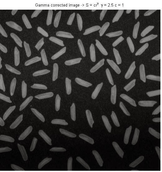
figure,imshow(S1);title('Gamma corrected Image -> S = cr^\gamma  \gamma = 0.40 c = 1');

Plots of the Equation:

%Power Law(Gamma) Transformation

GRng=[0.04; 0.10; 0.20; 0.40; 0.67; 1; 1.5; 2.5; 5.0; 10.0; 25.0];

R=0:255;

figure,

for i = 1 : 11

X=C*(R.^GRng(i));

Temp=256/X(256);

s=Temp*X;

plot(R,s);

title('Plot Equation S = Cr^\gamma');

xlabel('Input Intensity Level,r');

ylabel('Output Intensity Level,s');

text(R(175),s(175),['\gamma = ',num2str(GRng(i))],'HorizontalAlignment','left');

hold all

axis([0 255 0 255]);

end

EXPLANATION:

The transformation is plotted for different values of gamma for the intensity levels [ 0 255].

The output image intensity values are mapped to the range [0 255]